Equation \((\ref{eq:rendering_equation})\) shows the rendering equation and the precalculation which is stored in a lightmap is shown in Equation \((\ref{eq:lightmap_solution})\). The variable \(\mathbf{q}\) is a point retrieved through raycasting into the direction of light vector \(\mathbf{l}\). Looking at the equations it becomes apparent that the lightmap value is almost equivalent to the lighting integral but lacks the BRDF contribution, therefore it must be applied after the integration. Pulling the BRDF out of the integral is only valid if it is a constant term which restricts irradiance maps to Lambertian BRDFs.

$$ L_o (\mathbf{p}, \mathbf{v})= L_e + \int_{\mathbf{l}\in\Omega} f(\mathbf{l}, \mathbf{v})L_o(\mathbf{q}, \mathbf{-l})(\mathbf{n}_p\cdot \mathbf{l})^+d\mathbf{l}\tag{1}\label{eq:rendering_equation}$$

$$lightmap(x, y) = \int_{\mathbf{l}\in\Omega} f(\mathbf{l}, \mathbf{v})L_o(\mathbf{q}, \mathbf{-l})(\mathbf{n}_p\cdot \mathbf{l})^+d\mathbf{l} \tag{2}\label{eq:lightmap_solution}$$

The Lambertian BRDF is an acceptable approximation for body reflection of objects but a poor one for surface reflection. In consequence, it is impossible to decently precalculate the effect of highly specular objects using lightmaps.

The core of the light mapper is the solver which performs a Monte-Carlo integration. Before it can do that, the application generates so called charts which are texture regions which are mapped onto the static geometry, to do this the application may need to split a surface into multiple charts to allow a flattening of the geometrical surface. The vertices of each chart are then individually projected into a two dimensional space and textures which are large enough to store the projections are generated. Those textures are supposed to store a local lightmap for one chart only. A software rasteriser then generates fragments from the projected charts so that each of those fragments then represents a lightmap texel which corresponds to a surface point of the geometry. The attributes of the fragments are used as input into the integrator.

The Monte-Carlo integrator works iteratively, i.e. it solves all local lightmap texels for direct illumination first, then repeats to add indirect illumination after one bounce, then after two bounces and so on. This process continues for a user defined number of iterations.

When the integration terminates the individual local lightmaps needs to be combined and stored in a common texture. This process of joining all the individual lightmaps is called packing. A good packing helps reducing storage requirements of the lightmaps, so it is a crucial step for generating efficient lightmaps.

The following sections revisit each of the baker's stages and describe how they work in more detail.

Before storing any values, lightmap charts need to be generated. Each chart represents a continuous part of the scene's surface which has been projected into a 2D space and is mapped into the lightmap texture. It is much easier to perform this mapping if the surface represented by a chart is almost planar. This way there's no need to unfold geometry to prevent serious distortion of the surface, vertices can just be projected into lightmap space.

The algorithm of splitting the geometry into charts works as follows:

1. Add all primitives to a list \(L\)
2. Terminate if \(L\) is empty, otherwise pop a primitive \(p\) from \(L\)
3. Add all neighbors of \(p\) to a collection of potential chart primitives called \(P\) unless they are already member of a chart, add the primitive \(p\) to the list of primitives for the current chart \(C\)
4. If \(P\) is empty go to 2, otherwise pop a new \(p\) from list \(P\)
5. Determine average normal of current chart \(C\) as \(\mathbf{n}_{avg}\) and normal of \(p\) as \(\mathbf{n}_p\)
6. If \(\mathbf{n}_p\cdot\mathbf{n}_{avg} \geq t \ | \ t \leq 1\), \(p\)'s orientation is considered similar to the chart's orientation, therefore \(p\) is added to \(C\) and removed from \(L\)
7. The neighbors of \(p\) are added to \(P\) unless they are already in a chart; then repeat from 4.

This pseudocode in Listing 1 describes the algorithm more concisely.

The subsequent projection to lightmap space is then performed by first finding the component-wise minimum of the chart's vertex positions in model space, i.e. the smallest x, y and z-coordinates across all vertices. By subtracting this minimum from each chart vertex the chart's bounding volume minimum is \((0,0,0)^T\). These adjusted positions are then projected to two dimensions by projecting the position vectors of the vertices into a two dimensional orthonormal basis.

The first step of the projection is to find suitable axes for the new basis. Equations \((\ref{eq:basis_locallightmap1})\) and \((\ref{eq:basis_locallightmap2})\) show how to compute the directions \(\mathbf{x}^\prime\) and \(\mathbf{y}^\prime\) of these axes which then need to be normalised to form the basis vectors \(\mathbf{x}\) and \(\mathbf{y}\). The projection itself is shown in Equation \((\ref{eq:projection_locallightmap})\).

$$\begin{align}
\mathbf{x^{\prime\phantom{\prime}}} &= \mathbf{b} \ - \ \mathbf{a}\\
\mathbf{y^{\prime\prime}} &= \mathbf{c} \ - \ \mathbf{a}
\end{align}\label{eq:basis_locallightmap1}\tag{5}$$

Orthogonalising \(y^{\prime\prime}\) by computing
$$\mathbf{y^\prime} = \mathbf{y^{\prime\prime}} - (\mathbf{x}\cdot\mathbf{y^{\prime\prime}}) \mathbf{x}\label{eq:basis_locallightmap2}\tag{6}$$

$$\begin{align}
\mathbf{p}^L_x &= \mathbf{x}\cdot\ \mathbf{p}^W_x\\
\mathbf{p}^L_y &= \mathbf{y}\cdot\ \mathbf{p}^W_y
\end{align}\label{eq:projection_locallightmap}\tag{7}$$

The superscripts \(L\) and \(W\) denote local lightmap and adjusted world space coordinates respectively. This projection results in one isolated local lightmaps per chart. The solver will work with the local lightmaps because the required smoothing of the Monte-Carlo integrated irradiance values is simpler that way.

When the individual charts are in place, it must be determined which lightmap texels are covered by the chart primitives. This is equivalent to GPU rasterisation which determines all pixels covering screen pixels. Therefore, a simple software rasteriser is used for this task. Its simplicity comes from the fact that some steps required in a hardware rasteriser can be omitted. One example is perspective correction through division with w, which is possible because depth is irrelevant for rasterising charts.

The projected primitives are rasterised by scanning through the lightmap pixels in a zig-zag order. At each pixel centre the edge equation as shown in Equation \((\ref{eq:edge_equation})\) needs to be evaluated for each of the primitive's edges.

$$e_n(x, y) = -(v^a_y-v^b_y)x + ( v^a_x-v^b_x)y = \Delta x \cdot x + \Delta y \cdot y\label{eq:edge_equation}\tag{8}$$

Where \(n\) stands for the index of the edge, \(v\) represents a vertex of the primitive with the superscript denoting a vertex of the edge and the subscript indicating the component of a vertex' location vector. Care must be taken to plug edge vertices into the equation in the right order. Vertex \(a\) must come before \(b\) when ordering primitive vertices clockwise. The pixel is part of the primitive each time all edge functions evaluate to a positive number. The exact determination of when a pixel is covered by Akenine-Möller [AM07]T. Akenine-Möller. [Mobile] Graphics Hardware. Lunds Tekniska Högskola, 2007.
https://fileadmin.cs.lth.se/cs/Education/EDA075/notes/mGH.pdf

He also describes how to accelerate rasterising by solving these equations iteratively. This works because at each step in x-direction 1 is added to \(p_x\) and each step in the positive y direction 1 is added to \(p_y\). Thus, the following holds:
$$\begin{align}
e_n(x + 1,y) &= e(x, y) + \Delta x \\
e_n(x,y+1) &= e(x, y) + \Delta y
\end{align}\tag{9}$$

Further processing of the fragments requires interpolated normals and world space positions. Those are interpolated using barycentric coordinates as also shown by Akenine-Möller.

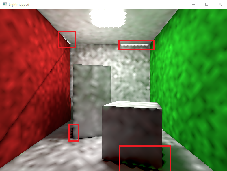
The fragments generated this way are not sufficient. If these fragments are shaded and stored in the lightmap there is a problem at texture lookup. The problem arises because the texture is usually not read exactly at the pixel centre and the neighboring texels are blended into the lookup result by a bilinear interpolation based on the lookup position, see Figure 1. For texels at a primitive's edge, such a texture access will blend unrelated texel colors into the result, i.e. the filtering footprint is larger than the actual projected chart. Figure 2 shows what this problem looks like. To prevent this the primitive must be dilated so that a guard band of one pixel in x and y direction is added. Currently this is done in a cumbersome way by keeping all fragments sorted by coordinates and adding all neighboring texels which don't create duplicates.

For very small charts it can be advatageous to skip part of the dilation to save texel storage. If a chart's extent in a dimension is less than the extent of one texel, the dilation in this dimension is omitted as descibed by [Bou13]M. Boulton. Static Lighting Tricks in Halo, 2013
https://www.gdcvault.com/play/1017902/Static-Lighting-Tricks-in-Halo
. This is possible because only one texel in that dimension holds all information required and therefore interpolation is useless. The interpolation is suppressed by clamping the lightmap's UV coordinates in that direction to the texel center.

The world space position of the individual fragments generated in the previous step are the geometry's surface points for which the rendering equation needs to be solved. To guarantee a good Monte-Carlo estimate of the lighting integral a set of rays with random directions over the hemisphere is required. The random directions can be generated in many ways, here points are sampled uniformly over a unit disk and then projected up onto the unit hemisphere. The vector from hemisphere centre to a hemisphere surface point is a unit direction vector. To uniformly distribure sample points over a unit disk in spherical coordinates, uniform random variables \(\xi_1\) and \(\xi_2\) need to be scaled [PH10]M. Pharr and G. Humphreys. Physically Based Rendering: From Theory to Implementation . Morgan Kaufmann, 2010 as shown in Equations \((\ref{eq:disk_sampling1})\) and \((\ref{eq:disk_sampling2})\).

$$\begin{align}
r &= \sqrt{\xi_1}\tag{4}\label{eq:disk_sampling1}\\
\theta &= 2\pi\cdot\xi_2\tag{5}\label{eq:disk_sampling2}
\end{align}$$

These sample points are then converted to cartesian coordinates by Equations \((\ref{eq:disk_to_hemisphere_x})\) to \((\ref{eq:disk_to_hemisphere_z})\) . The points are easily projected on the hemisphere in Cartesian coordinates by investigating the length of the sample location vectors. The y coordinate must be set in such a way that the length of the vector becomes 1 which is done by solving \(y = \sqrt{1-x^2-z^2}\).

$$\begin{align}
x &= r\cdot\sin\theta\tag{6}\label{eq:disk_to_hemisphere_x} \\
y &= 0\tag{7}\\
z &= r\cdot\cos\theta\tag{8} \label{eq:disk_to_hemisphere_z}\\
\end{align}$$

This procedure generates the samples in tangent space with the y-Axis being equivalent to the surface's normal. The solver however, needs these samples in world space so the coordinates need to be transformed by a change of basis matrix which provides this mapping. The conversion from tangent to world space is a transformation from one orthonormal basis into another orthonormal basis and can be formulated by a single matrix multiplication \(x^W = Mx^T\), where the superscript indicates world or tangent space. The change of basis matrix \(M\) is constructed by finding the orientation of the tangent space basis vectors in world space. These vectors correspond to the surface's normal, tangent and bitangent. The location of a point in world coordinates can be obtained by projecting a point on the three basis vectors through a dot product and using the results as the corresponding vector components. This can be done by a matrix multiplication with \(M\) if the matrix is composed with the basis vectors as row vectors.

The correct irradiance values are determined by performing the integration from the rendering equation. Since this cannot be done analytically a numerical solver is needed. The most popular method to solve the equation is to employ a kind of Monte-Carlo integration. Here a plain Monte-Carlo integration is used even though results would converge faster to the correct solution by introducing importance sampling.

As mentioned before the equation is solved iteratively by solving each light bounce individually. To do this, the integrator takes the lightmap fragments and generates a set of directions in the hemisphere for this point. Each of the resulting rays then needs to evaluate how much irradiance is contributed from the direction they represent. This radiance must come from another object in the scene, either through reflection or emitted by that objects surface. Therefore the first intersection point of the ray with the scene needs to be determined.

This first intersection point is found by consulting an acceleration structure which returns a set of candidate primitives. The structure itself is described in more detail in a dedicated section below. The solver then evaluates each of the candidate primitives by first finding the intersection point of the ray with the primitive's plane. The location of a ray-plane intersection point of ray \(\mathbf{x} = r_0 + t\mathbf{d}\) and plane \(\mathbf{n}\cdot\mathbf{x} = \mathbf{p_0}\) is found by solving Equation \((\ref{eq:rayplane_intersection})\) for \(t\) which results from substitution of \( \mathbf{x}\) in the ray and plane reperesentation.

$$t = \frac{
( \mathbf{p_0} - \mathbf{ r_0})\cdot\mathbf{n}
}{
\mathbf{d}\cdot\mathbf{n}
}\tag{8}\label{eq:rayplane_intersection}$$

The intersection point retrieved this way is then converted into barycentric coordinates of the primitive by using the Equations \((\ref{eq:convert_barycentric1})\) through \((\ref{eq:convert_barycentric3})\). [Eri04]C. Ericsson. Real-Time Collision Detection, The Morgan Kaufmann Series in Interactive 3-D Technology . CRC Press, 2004

$$
\begin{align}
v &= \frac{
\mathbf{d_{11}}\cdot\mathbf{d_{20}}-
\mathbf{d_{01}}\cdot\mathbf{d_{21}}
}{
\mathbf{d_{00}}\cdot\mathbf{d_{11}}-
\mathbf{d_{01}}\cdot\mathbf{d_{01}}
}\tag{9}\label{eq:convert_barycentric1}\\[5px]
w &= \frac{
\mathbf{d_{00}}\cdot\mathbf{d_{21}}-
\mathbf{d_{01}}\cdot\mathbf{d_{21}}
}{
\mathbf{d_{00}}\cdot\mathbf{d_{11}}-
\mathbf{d_{01}}\cdot\mathbf{d_{20}}
}\tag{10}\label{eq:convert_barycentric2}\\[5px]
u &= 1 - u - w\tag{11}\label{eq:convert_barycentric3}
\end{align}
$$

Where the individual variables are defined as:

$$
\begin{align}
\mathbf{v_0} &= \mathbf{B} - \mathbf{A}\\
\mathbf{v_1} &= \mathbf{C} - \mathbf{A}\\
\mathbf{v_2} &= \mathbf{P} - \mathbf{A}\\
\mathbf{d_{00}} &= \mathbf{v_0}\cdot \mathbf{v_0}\\
\mathbf{d_{01}} &= \mathbf{v_0}\cdot \mathbf{v_1}\\
\mathbf{d_{11}} &= \mathbf{v_1}\cdot \mathbf{v_1}\\
\mathbf{d_{10}} &= \mathbf{v_2}\cdot \mathbf{v_0}\\
\mathbf{d_{21}} &= \mathbf{v_2}\cdot \mathbf{v_1}\\
\end{align}
$$

With \(A,B\) and \(C\) being the primitive's vertices and \(P\) the intersection point. The barycentric coordinates allow to determine if the intersection point is contained in the primitive, by verifying if they fulfil the following conditions:

• \(0 \leq u \leq 1\)
• \(0 \leq v \leq 1\)
• \(0 \leq w \leq 1\)

If there is no intersection of the ray with any geometry the radiance through this ray is set to 0. If however, the intersection point is inside the primitive, the barycentric coordinates can be used to interpolate the texture coordinates retrieved from the primitives vertices. The interpolated coordinates are then used to fetch the radiance value stored in the lightmap.

The irradiance contributed by this ray is then the fetched radiance weighted by the BRDF and the cosine term plus radiance emitted by the primitive. Irradiance is determined this way for the whole set of rays generated and are then used for the Monte-Carlo integration. Recall that a Monte-Carlo integration approximates an integral by solving for a few samples which are averaged and then scaled to the whole domain. Doing so for the unit hemisphere results in Equation \((\ref{eq:integration_montecarlo})\).

$$E(\mathbf{p})=\frac{2\pi}{N}\sum_{r \in R} L_o(raytrace(\mathbf{p}, \mathbf{r}), -\mathbf{r})\label{eq:integration_montecarlo}\tag{3}$$

In this equation \(raytrace(\mathbf{p}, -\mathbf{r})\) represents the location of the first intersection of the ray and \(\mathbf{p}\) is the surface point retrieved from the lightmap texel so that \(L_o\) is the result from the ray test. \(E(\mathbf{p})\) is the solution of the rendering equation for this iteration at point \(p\) and therefore stored in the lightmap.

This process is repeated for each lightmap fragment and for each iteration. This way each iteration \(i\) adds contibution of radiance that was bounced \(i\) times beginning with only direct illumination in the first iteration. Experience shows that after only a few bounces irradiance approaches the correct solution close enough to have convincing illumination as each bounce influences the scene less than the previous bounce.

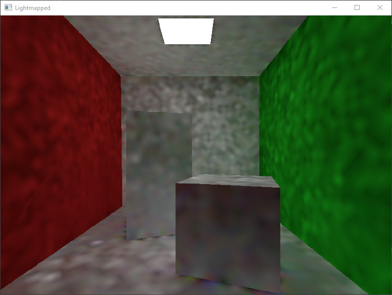
At this point there are local light maps available which contain the Monte-Carlo integrated irradiance after a number of bounces. Due to the integration method there is some noise in the lightmaps which is clearly visible as can be seen in Figure 3. The noise can be reduced by smoothing the irradiance map with a Gauss-like filter. Since the filter must preserve chart edges a pure Gaussian filter is unsuitable but a bilateral filter provides the required smoothing and edge preservation. The input to the filter is only the irradiance map, the parameter which determines texel weight is the texture's alpha value which was set to 1 when writing to the lightmap.

Bleeding of irradiance between two adjacent charts is prevented by keeping the chart's irradiance local lightmaps until now. After the smoothing took place the common lightmap can be merged into one global lightmap.

The final step of the lightmapper is to assemble a global lightmap from the individual local lightmaps. For production, packing efficiency and speed are most important, in this sample application there was no extra effort spent on optimizing the packing process. Nonetheless, the process shouldn't waste too much texture space without reason. The packing is a brute force approach similar to the one presented in [Bou13]M. Boulton. Static Lighting Tricks in Halo, 2013
https://www.gdcvault.com/play/1017902/Static-Lighting-Tricks-in-Halo

The final position of a chart is found by the following algorithm: Originally the chart is assumed to be placed at the top left of the lightmap and for each texel of a chart it is checked if the destination texel is within lightmap bounds and unoccupied. The vacancy of a position is stored in the alpha channel as value 0. If this check determines that the chart cannot be placed at the current position, the chart's offset is updated. First the x coordinate of the chart offset is increased, unless this exceeds the lightmap's dimension in x-direction or the algorithm tries to place a texel outside the x-dimension. In that case the y-offset is increased and the x-offset is reset to 0. The map is considered full as soon as the offset exceeds the lightmap's y-range. In this situation it would be possible to either create a second map which is being filled or resizing the current lightmap but this application will only generate one fixed size lightmap and will fail when the lightmap is full.

It shouldn't be surprising that solving the rendering equation takes quite some time as there is a large number of rays which need to be evaluated for each surface fragment generated in the rasteriser stage. Therefore a lookup structure is introduced which is supposed to accelerate ray intersection testing. Without support of an acceleration structure each ray must be tested against every primitive in the scene. This is obviously very wasteful as it processes primitives even if a ray can't possibly intersect it, such as primitives behind the ray's initial point. The lookup structure will reduce the number of primitives to a small number of candidate primitives which the ray might intersect.

The structure presented in [Kar12]T. Karras. Thinking Parallel, Part III: Tree Construction on the GPU, 2012
https://devblogs.nvidia.com/thinking-parallel-part-iii-tree-construction-gpu/
has been reproduced for this application. The basic idea is to sort all geometric primitives by its morton order. This number represents a cell of a grid by an index in such a way that the cells of ascending morton order follow a z-curve, such a curve is shown in Figure 5. Finding this z-order of a primitive is simpler than it appears: First the cell index in x, y, and z-direction is determined independently by simply discretising space in each dimension. This order must be stored as unsigned integer for the next step to work. The individual indices are then combined by interleaving the individual bits of the according variables with each other in a XYZ order. This is done by inserting two zeros between each bit first, then left shifting x by 2 bits and y by 1 bit before eventually bitwise ORing the three numbers. The expansion can be done by cleverly manipulating the bit patterns as shown in Listing 2.

After determining the morton order of each primitive, an array of all order values is sorted in ascending order. The arrays holding primitive ID and bounding box information are sorted as well to keep the information in sync, that is the morton order stored at array index i has its primitive ID and bounding box also stored at index i in the corresponding array. With these sorted arrays the actual hierarchy can be built. The actual code to build the hierarchy is shown in Listing 3.

The basic idea of the algorithm is that each bit position of the morton code effectively splits a subvolume of the hierarchy into two halves. For the lower half the according bit is 0 and for the upper half it is 1. The MSB splits the total volume into two halves in x direction, the following bit splits those two halves into two subvolumes in y direction etc. This follows directly from the definition of the morton codes.

The outer loop of the algorithm iterates over the range of morton codes representing a volume, retrieves bit position b at which the parent volume had been split and finding the index of the first value which has the bit position b = b + 1 set to 1. This index represents the volume's split position and can be found using a binary search since the morton codes are sorted. It is possible that there is no split position for the current bit position, in this case b is increased until a valid split position is found or the LSB was checked.

The vector counting_subvols in the code snippet keeps track of the current volume's parents so that the subvolume counter of the parents can be updated each time new volumes are inserted. The subvolume counter value represents the number of volume entries in the output arrays between the parent and its next sibling so that all descendants of a volume can be skipped at once.

When a volume is split, it is added to the stack of parents, all parent's subvolume counters are increased by 2 and the two new subvolume ranges are added after the volume range being split. The stored range also saves the bit position at which this split occured. If the split index coincides with the last index of one or more ancestor volumes, those ancestors cannot have other descendants which haven't been split yet. Therefore they are removed from the list of ancestors, the loop variable is increased and the next iteration begins over sibling of the last ancestor that was removed.

Since new volumes are added after their parents, the algorithm will split those before advancing to a sibling of the parent volume. This behaviour is similar to a depth first search and necessary to count descendants correctly.

The output of the function is a structure holding arrays for the axis aligned bounding box (AABB) extents, associated primitives and the skip values. The primitive information holds a starting index and number of primitives per volume which refer to another array holding the morton order sorted primitive IDs. This setup allows to iterate over the AABB array and test for ray intersection with it. If an AABB is not intersected the iteration can skip all descendants because the number of descendants is stored in the skip value.

The biggest problem currently is that the effectiveness of the acceleration structure cannot be evaluated properly. The test scene is simply too small to make a perceivable difference.

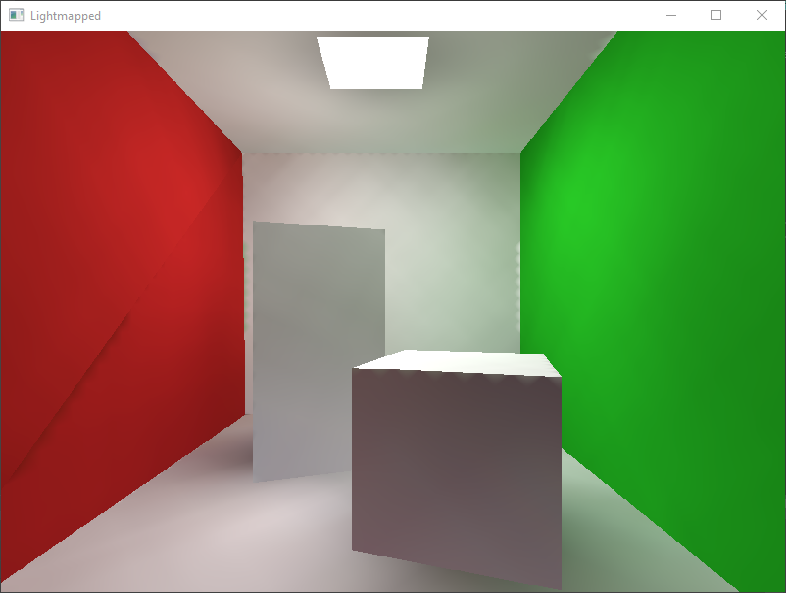
Visually the largest problem is that neighbouring geometric elements which are solved individually, e.g. at locations where the chartmap is split or where a primitive is adjacent to another without sharing vertices, expose clearly visible seams. This can be seen on the red face face in Figure 4 because this face doesn't share vertices. These seams can be fixed relatively simple as described in [Iwa13]M. Iwanicki. Lighting Technology of "The Last of Us", 2013
http://miciwan.com/SIGGRAPH2013/Lighting%20Technology%20of%20The%20Last%20Of%20Us.pdf
but hasn't been implemented yet. Another visible issue occurs at chart edges, where neighboring charts can leak into each other. The problem there is that the rasterising step needs to rasterise conservatively to ensure that the whole triangle area is contained by the resulting fragments. This shortcoming also defeats the triangle dilation in the rasterising step as the filter footprint. However, the dilation hides the issue in many cases.

A way of accelerating the solution may be to reuse the generated rays and simply rotating the sample kernel about the surface normal for neighbouring lightmap texels, similar to how it is done in many screen space ambient occlusion solutions. The effect of doing so may be neglectible though.

The time intensive solution of the rendering equation makes a parallelisation of the light mapping process interesting and the nature of the solver lends itself for good parallelisation as each ray and each lightmap texel that needs to be solved for is completely independent. This opimisation has not been explored because it makes more sense to move to the GPU first as it allows to use even more threads. In this case care must be taken that each thread's workload is similar enough to prevent thread divergence. Alternatively the support of hardware ray tracing capabilites can be exploited.

From a supported feature perspective it is relatively simple to extend the current solution to support radiosity normal maps as it merely stores more information that is already available in a number of textures. Radiosity normal maps store outgoing radiance in the directions of three axes forming a orthonormal basis in tangent space. The additional information allows to interpolate outgoing radiance in any direction so that arbitrary BRDFs can be used. This is also a quite old method which was developed by Valve for Half-Life 2 [MMG06]J. Mitchell, G. McTaggart and C. Green. Shading in Valve's Source Engine, 2006
https://steamcdn-a.akamaihd.net/apps/valve/2006/SIGGRAPH06_Course_ShadingInValvesSourceEngine.pdf
Adding more advanced storage as light probes requires more effort.