Skin Rendering with Texture Space Diffusion
Rendering human skin realistically poses the challenge of solving subsurface lighting sufficiently correct. This challenge is quite diffcult for skin due to its slight transluceny. This causes light entering the material to be scattered within and travel relatively long distances before exiting again. This distance then corresponds to more than a pixel's width of the final image. In this case the effect of subsurface scattering cannot be approximated with a simple BRDF like the Lambertian BRDF. Thus another way to incorporate subsurface scattering is required and multiple ways of solving the problem have been proposed. One of these algorithms is subsurface scattering which has the advantage of being relatively simple to implement but is also less performant than screen space [NP13]D. Neubelt and M. Pettineo. Crafting a Next-Gen Material Pipelnie for The Order: 1886, 2013
http://cdn.rtgfx.com/papers/s2013_pbs_rad_notes.pdf
.
The basic idea is to unfold a mesh to a planar surface by using the texture coordinates as positions, calculating irradiance at each location and then performing the diffusion of light, caused by subsurface scattering, over the resulting 2D texture. The diffusion follows a complex dipole diffusion function which can be approximated through a series of Gaussian filters though. After the convolution the resulting diffusion is applied to the final mesh in a separate render pass which also adds surface reflection for the final appearance of the object. The project presented here takes a lot from the corresponding GPU Gems chapter [DEonL07]E. D'Eon and D. Luebke. Advanced Techniques for Realistic Real-Time Skin Rendering, 2007
https://developer.nvidia.com/gpugems/gpugems3/part-iii-rendering/chapter-14-advanced-techniques-realistic-real-time-skin
which in turn is based on [DEonLE07]E. D'Eon, D. Luebke and E. Enderton. Efficient Rendering of Human Skin, 2007
.
Diffusion Profile Approximation
A good way to approximate the diffusion is described in [WJRMLH01]H. Wann Jensen, S. R. Marschner, M. Levoy and P. Hanrahan. A Practical Model for Subsurface Light Transport, 2001
https://graphics.stanford.edu/papers/bssrdf/bssrdf.pdf
which uses a dipole approximation, using a positive and a negative light source as poles, to calculate subsurface light transport. The diffusion function from that publication is shown in Equation $(
ef{eq:diffusion_term})$. The important bit is the diffusion profile which determines the result of the diffusion.
$$
S_d(x_i, \omega_i, x_o, \omega_o) = \frac{1}{\pi}F_t(\eta, \omega_i)R_d(\|x_i - x_o\|) F_t(\eta, \omega_o)\tag{1}\label{eq:diffusion_term}
$$
The diffusion profile is denoted as $R$ in Equation $(\ref{eq:diffusion_term})$ and is characteristic for materials exposing subsurface scattering behaviour such as skin. The paper and this forum post provide a lot of information about the whole approach.
The observation of [DEonLE07]E. D'Eon, D. Luebke and E. Enderton. Efficient Rendering of Human Skin, 2007 is that such a dipole profile can be approximated using a sum of weighted Gaussians which is advantageous as Gaussians are significantly less complex, allowing to compute light diffusion at much lower cost. Fitting a sum of Gaussians to the actual profile requires an error function to minimise against. The proposed error function is shown in Equation $(\ref{eq:fitting_error})$. Where G represents the individual Gaussians and w_i is a weighting. The variable r is distance of entry and exit points, i.e. $\|x_i - x_o \|$ from the diffusion function. This parameter is also used to scale the mean squared error to account for the larger circumference of the resulting circle over which the integration takes place.
$$
E = \int_0^\infty r \left(R(r) - \sum w_i G(v_i, r)\right)^2 dr\label{eq:fitting_error}\tag{2}
$$
The GPU Gems article presents a fitting of a sum of six weighted Gaussians for white skin. The weights were adjusted individually for each color channel to account for wavelength dependency of subsurface scattering distances. The weights and variances found are listed in Table 1:
Variance Red Green Blue 0.0064 0.233 0.455 0.649 0.0484 0.100 0.336 0.344 0.187 0.118 0.198 0 0.567 0.113 0.007 0.007 1.99 0.358 0.004 0 7.41 0.078 0 0
These Gaussian filters are applied in series, i.e the convolution of one blur pass is the input for the next pass. The detailed process is described below in a dedicated section.
Heightmap to Normals and Mip-mapping Heightmap
The head mesh applied is a head scan of Lee Perry-Smith obtained from Morgan McGuire's Computer Graphics Archive and comes with a height map which needs to be converted to normals. The generation of normals is done on the fly in the fragment shader using an algorithm presented in [And07]J. Andersson. Terrain Rendering in Frostbite Using Procedural Shader Splatting, 2007
https://developer.amd.com/wordpress/media/2013/02/Chapter5-Andersson-Terrain_Rendering_in_Frostbite.pdf
. The derivation is shown here and is based on the fact that the normal of an implicitly defined surface of the form $f(x, y, z) = c \ $ is defined as the gradient $\nabla f = \left(\frac{\partial f}{\partial x}, \frac{\partial f}{\partial y}, \frac{\partial f}{\partial z}\right)$ of that surface.
A hightmap as provided can be interpreted as the implicit function $h(x, y) - z = 0$ of which the partial derivatives need to be determined. The partial derivatives with respect to x and y are obtained by applying simple central differences and the one of z can be found analytically. This leads to the formula shown in Equation $(\ref{eq:gradient_heightmap})$.
$$
\nabla f = \begin{pmatrix}
\frac{h(x + 1, y)-h(x - 1, y)}{2}\\
\frac{h(x, y + 1)-h(x, y - 1)}{2}\\
-1
\end{pmatrix}\tag{3}\label{eq:gradient_heightmap}
$$
Since z is -1 the resulting normal is going to point below the surface and the vector must be flipped to have the desired tangent space normal. This is done by inverting the individual components which can already by done at the gradient derivation step. To lose any fractions the whole term is multiplied by 2 as the normal needs to be normalised afterwards anyway. The final normal is therefore computed in Equation $(\ref{eq:normal_heightmap})$ as shown by [And07]J. Andersson. Terrain Rendering in Frostbite Using Procedural Shader Splatting, 2007
https://developer.amd.com/wordpress/media/2013/02/Chapter5-Andersson-Terrain_Rendering_in_Frostbite.pdf
.
$$
\mathbf{n} = \begin{pmatrix}
h(x - 1, y)-h(x + 1, y)\\
h(x, y - 1)-h(x, y + 1)\\
2
\end{pmatrix}\tag{4}\label{eq:normal_heightmap}
$$
The actual shader code is shown in Listing 1
The issue with the resulting normal is that it has been constructed in tangent space and the vectors required to calculate lighting are in world space. A transformation from world space to tangent space is carried out by dotting the normal vector the world space representation of te individual tangent space basis vectors. This can be expressed as a matrix multiplication by the matrix
$$M = \begin{bmatrix}
t_x & t_y & t_z\\
b_x & b_y & b_z\\
n_x & n_y & n_z\\
\end{bmatrix}$$
The issue at this point is that a surface normal for the current primitive is known but there is no tangent provided. A tangent can be obtained as described by [Sch13]C. Schueler. Followup: Normal Mapping Without Precomputed Tangents, 2013
http://www.thetenthplanet.de/archives/1180
. The core of this method is the observation that the gradients of texture coordinates provide vectors in tangent space which can serve as tangent and bitangent. The resulting basis is most often not orthonormal but that is not a problem for the transformation. The gradient calculation provides the possibility of creating an underdetermined system of linear equations, if rearranged as in Equation $(\ref{eq:to_linequations})$.
$$
\mathbf{t} = \nabla u = \frac{dp}{du} \rightarrow du = \mathbf{t} \cdot dp\\
\mathbf{b} = \nabla v = \frac{dp}{dv} \rightarrow dv = \mathbf{b} \cdot dp\label{eq:to_linequations}\tag{5}
$$
Since the differentials of a single primitive result from a linear interpolation of vertex attributes they are constant over the primitive surface. This allows to use the texture coordinate differences between the individual vertices directly which results in the two equations for the system of linear equations in Equation $(\ref{eq:underdetermined_sle})$.
$$
\Delta u_1 = \mathbf{t} \cdot \Delta p_1
\Delta u_2 = \mathbf{b} \cdot \Delta p _2\label{eq:underdetermined_sle}\tag{6}
$$
A unique solution requires a third equation which can be derived from the fact that bitangent and tangent have to be orthogonal to the normal which means that the dot product of the tangent with the normal must be 0. The tangent space normal is obtained by the cross product of the positional differences which results in Equation $(\ref{eq:determining_equation})$ so that the system is now determined.
$$
0 = \mathbf{t} \cdot \Delta p_1 \times \Delta p _2\label{eq:determining_equation}\tag{7}
$$
A final problem with the heightmap is mip mapping. A simple way to apply another mip level is to create a trilinear sampler which automatically selects the correct level. The issue that arises is that central differences needs the coordinates of the neighbouring texels and since those are always in the range [0,1] they are dependent on texture dimensions of the mip level used. Simply using the highest level effectively defeats the use of mip mapping which results in objectionable noise in the normal field and therefore in lighting. This issue is addressed by manual calculation of the mip map level via the intrinsic derivative functions so that the derivatives of that specific level are used.
Mip map levels are selected to approach a texel to screen pixel ratio as close to 1:1 as possible. The texture coordinates u and v are in the range $R \in [0, 1]$ and the fraction of that range covered by one screen pixel in x and y direction is given by the respective derivatives dx and dy of the uv coordinates. Knowing this fraction, it is trivial to calculate the optimal texture size by dividing the full range by the fraction. The result is the number of texels the correct mip map level should have and the mip map level L is then calculated using log2. Since there are derivatives in x and y direction a decision about the derivative to use has to be made, here the larger derivative is chosen to calculate the correct mip level. The whole determination is formalised by Equation $(\ref{eq:miplevel_determination})$. The final -1 in that equation is needed to account for zero-based indexing.
$$
\begin{align}
d_{max} &= \max\left({\left\|\frac{duv}{dx}\right\|, \left\|\frac{duv}{dy}\right\|}\right)\\[10px]
L &= L_{max} - \log_2\left(\frac{1}{d_{max}}\right) - 1\tag{8}\label{eq:miplevel_determination}
\end{align}
$$
And here is the corresponding HLSL code:
Generating Shadow Map
The shadow map used in the presented approach is an extended translucent shadow map (TSM) which stores the models UV coordinates in addition to light source distance and mesh normals. The need to store more than depth values forces a draw to a render target in order to store all information as opposed to regular shadow maps for which a depth write is sufficient. The values are obtained as in ordinary shadow maps: The mesh is rendered from the point light source's position using a perspective projection and UVs, view space depth and view space normals are written. Since this setup needs 6 floats to be stored the shadow pass makes use of multiple render targets (MRT). For high quality shadow maps the light frustum should be fit to enclose shadow receivers as closely as possible before the actual drawing. This can be omitted here as there is only one receiver at a constant distance and the light frustum is always focused on this single object. This and the objects shape result in a situation where the closest fit is almost constant and the frustum doesn't need to be adjusted given a certain guard band around the object in the shadow map. This reasoning allows the light's projection matrix to be hardcoded.
For efficiency it is useful to pack the normal and depth value into one render target because those are all values needed for the irradiance pass. This way one 4 channel texture read is sufficient during irradiance map generation. Unfortunately this wastes two channels in the other render target as all render targets using MRT need the bit depth. Eventually a second texture read may be worth the cost to save those two channels but this has not been tested.
Figure 1 shows the resulting shadow map targets for a light position.

Generating Irradiance Map
The generation of irradiance maps and convolutions of it is the core of the algorithm. Irradiance maps store irradiance of light which is subject to body reflectance, i.e. light which was reflected at the surface is not considered. This kind of reflection is usually approximated using a simple BRDF, often a simple Lambert term $\frac{\rho}{\pi}$. Such a crude approximation is possible because subsurface scattering occurs over very small distances which appear less than a pixel wide on the screen.
For human skin these scattering distances are larger so that this approximation does not hold and subsurface scattering needs to be addressed explicitly. The irradiance map serves as a basis to approximate the effect of large distance subsurface scattering. Creating an irradiance map is rather straightforward, all that needs to be done is to unfold a mesh into a two dimensional representation by using available UV coordinates as world space coordinates in a vertex shader and then processing those positions as usual. Lighting is then calculated as for any other object. In this case Schlick's Fresnel term is used to subtract radiation which has already been reflected at the surface. Doing so is not energy conserving and therefore physically incorrect but results are acceptable anyway. For an energy conserving solution irradiance needs to be weighted as shown by [KSK01]C. Kelemen and L. Szimay-Kalos. A Microfacet Based Coupled Specular-Matte BRDF Model
with Importance Sampling, 2001
http://cg.iit.bme.hu/~szirmay/scook.pdf
as it has been done in the original presentation of this algorithm. The body reflected radiance is then scaled using the Lambertian BRDF while the albedo value used in this process is the square root of the value stored in the albedo map to implement pre- and post scattering as described by [DEonL07]E. D'Eon and D. Luebke. Advanced Techniques for Realistic Real-Time Skin Rendering, 2007
https://developer.nvidia.com/gpugems/gpugems3/part-iii-rendering/chapter-14-advanced-techniques-realistic-real-time-skin
. Another square root of the albedo map is later multiplied into the result during the final render pass. Eventually, an simple unmodified ambient radiance constant is added for the final result.
During convolution of irradiance values, thickness of material towards the light source should be convolved as well. The reasoning behind this is that very small features should not create large sudden responses as that would cause artifacts. This parallel convolution is achieved by storing material thickness in the alpha channel of the irradiance map, so this value needs to be calculated during irradiance map computation.
Evaluation of material thickness is derived for a case of parallel planar surfaces as shown in Figure 2. The point to be shaded is point C in the image but determining thickness at point B is much simpler. This point is guaranteed to either be close to C or the dot product $(n \cdot l)$ is going to be very small which reduces the effect of an incorrect approximation by a lot.
If the fragment to be shaded is illuminated frontally there is no light from the back to shine through. For this case the thickness should be set to a high value which won't allow any radiance to pass through. This way one can simply apply thickness without making this distinction later. A fragment is lit frontally if the dot product $(n \cdot l)$ is positive.
Determining the distance d between the points A and B is done via the distance between A and C. The length of AC is estimated by taking the fragment to light distance and then subtracting the depth value stored in the shadow map. Care must be taken to guarantee that all values are in the same space, therefore light position, fragment position and depth value are all stored in view space. A multiplication with the cosine of the angle between the back side's normal and the light vector yields d. Since the normal on the back is not known the assumption of parallel planes is exploited and the inverted normal of the current fragment can be used. Instead of using the inverted normal the relationship $(-a \cdot b) = -(a \cdot b)$ is applied and the dot product is inverted.
Since the surfaces are not always parallel planes the final thickness value is a linear interpolation of the unscaled and scaled thickness with an interpolator which estimates planarity. This estimate is simply the dot product of the fragment's inverted normal and the normal stored in the shadow map.

Listing 3 shows the whole calculation of thickness:
Before diffusion can be applied to the irradiance map, texture space distortion needs to be addressed. This distortion occurs because the texture is stretched and squeezed to fit onto the mesh and is a problem when filtering in texture space, as uniform distances in texture space do not correspond to uniform distances on the mesh. To work around this limitation a stretch map is generated by looking at the screen space derivatives of object space positions (the positions derived from the mesh's vertex coordinates rather than the transformed UV-coordinates). In [DEonLE07]E. D'Eon, D. Luebke and E. Enderton. Efficient Rendering of Human Skin, 2007 a simple inverse of the derivative is used as in Equation $(\ref{eq:stretch_simple})$. This is supposed to lie mostly within the range [0, 1] and should be scaled into that range with a hand tuned factor if necessary.
$$
S =
\begin{pmatrix}
\frac{1}{\left|\frac{dP}{dx}\right|}\\
\frac{1}{\left|\frac{dP}{dy}\right|}
\end{pmatrix}\tag{9}\label{eq:stretch_simple}
$$
The model used here creates stretch values far beyond 1 using this method which means that another method to determine distortion needs to be found. An alternative is to relate the screen space derivative of object space position to the screen space derivative of texture coordinates as shown in Equation $(\ref{eq:stretch_correlated})$ which resolves the issue completely.
$$
S =
\begin{pmatrix}
\frac{ \left|\frac{dUV}{dx}\right|}{\left|\frac{dP}{dx}\right|}\\
\frac{\left|\frac{dUV}{dy}\right|}{\left|\frac{dP}{dy}\right|}
\end{pmatrix}\tag{10}\label{eq:stretch_correlated}
$$
This is done in HLSL and written to a RGBA texture as shown in Listing 4
Diffusion using Gaussians
With irradiance and stretch maps at hand the actual diffusion can be approximated. This is done by convolving the irradiance map in series. This serial convolution exploits the fact that the convolution of two weighted Gaussian filters is expressed by the relation in Equation $(\ref{eq:gaussians_convolved})$.
$$
G(v_1, r) \ast G(v_2, r) = G(v_1 + v_2, r)\tag{11}\label{eq:gaussians_convolved}
$$
Another useful property of Gaussians is separability which allows to perform horizontal convolution first, followed by a separate vertical convolution pass which reduces the number of required texture reads significantly, from r² to 2r, where r is the filter radius. The convolution is applied not only to the irradiance map but also to the stretch map. This is done to prevent small features from impacting the irradiance convolution disproportionately. The stretch map convolution is works exactly as the irradiance convolution but happens right before irradiance manipulation, i.e. first the stretch map is convolved and then the irradiance map is convolved using the result of that stretch map convolution.
The actual convolution is carried out by reading the convolved stretch map at the convolution position as the central tap and generating a number of equidistant taps around this center with a spacing of one texel. This spacing is then scaled by standard deviation (SD, calculated from supplied variance) and stretch map value. The weights per sample are the weights of a standard normal distribution P(x) at the original texel distances so that for a 7 tap filter the weights are the values for P(-3), (-2), P(-1), P(0), P(1), P(2), P(3). This is done once in horizontal and then in vertical direction to make use of the advantages of separability and is applied to irradiance and stretch map in the exact same way, i.e. the stretch map modifies its own convolution.
The shader code below performs the convolution and also normalises the result by the total weight. The shader is responsible for horizontal convolution only. Vertical convolution is almost the same, the difference being that all values in x direction are replaced with values in y direction.
Final Render Pass
The final render pass combines the results of the individual convolutions with the surface reflectance and effects of translucency in thin body parts such as ears or nostrils. The combination of body and surface reflection is straightforward as both terms are simply summed. Surface reflection is calculated using any physically based rendering specular BRDF and body reflectance is computed by reading the individual convolved irradiance maps and weighting the stored irradiance with the diffusion profile weights before summing them up. The twist of adding body reflectance is to combine the diffused part of albedo with the part of albedo that had been separated by taking a square root before convolving irradiance. This is done by simply multiplying the convolved part with the square root of the albedo map, effectively reversing the square root.
Adding translucency is a little more involving but also not too difficult as thickness of the object has already been estimated. This thickness is now used in conjunction with irradiance stored on the backside of the visible object. These irradiance values are queried by looking up the irradiance map's UV-values in the shadow map. So the process works as follows: The current fragment's position is transformed into light space and the resulting normalised device coordinates need to be transferred into UV-coordinates of the shadow map. Using these coordinates the corresponding texel is fetched from the shadow map which holds another set of UV coordinates representing the irradiance map texture coordinates visible to the light. Those latter UV coordinates are then used to fetch the actual backside's irradiance value. As radiance is also attenuated while travelling through material the resulting value needs to be convolved again using the estimated thickness at the visible surface, i.e. the thickness needs to be fetched directly with the fragment's associated UV coordinates and not through a redirection via the shadow map. The final convolution is then approximated by Equation $(\ref{eq:translucent_diffusion})$, where $d$ is equivalent to the thickness value, $w_i$ are the diffusion profile weights and $v_i$ the diffusion profile variances.
$$
R(\sqrt{r^2 + d^2}) = \sum_{i=0}^k w_i G_i (v_i, \sqrt{r^2 + d^2}) = \sum_{i=0}^k w_i e^{-d^2/v_i} G(V_i, r)\tag{12}\label{eq:translucent_diffusion}
$$
Performance Considerations
The presented method has major disadvantages with respect to performance due to a few reasons: First, it needs to render each object which is subject to subsurface scattering into an offscreen texture and processes the results individually. This means a lot of overhead for scenes which contain a large amount of such objects, e.g. a scene with many characters visible on screen. This drawback is exacerbated by the fact that rendering lighting into offsecreen textures removes the opportunity for optimising performance through backface culling as each triangle is necessarily front facing. On top of that these irradiance textures need to be convolved five times while each convolution requires a two passes for horizontal and vertical convolution and each of these require many texture fetches which degrade performance significantly.
In [HBH09]J. Hable, G. Borshukow and J. Hejl. Fast Skin Shading, 2009 , John Hable et al. describe ways to work around some of the limitations of the original texture space diffusion approach. They improve on the culling issue by masking back facing primitives via the depth buffer, i.e. back facing primitives write a high value into the depth buffer so that rendering a full screen quad during the blur pass with depth testing enabled saves shader invocations for those faces.
Another improvement described by them is the use of a more compact sampling pattern to perform the blur. They achieve the five Gaussian convolutions by approximating the blur using 13 texture samples in a single pass. Their derivation of the tap weights is derived from the sum of five Gaussians described in [DEonLE07]E. D'Eon, D. Luebke and E. Enderton. Efficient Rendering of Human Skin, 2007
and the sampling pattern has been determined by defining two concentric rings representing mid distance and long distance subsurface scattering which are divided into six individual regions. A jittered sample is then placed in each region and at the center of the two rings. The need of rendering each relevant object into an irradiance map is completely avoided by [JSG09]J. Jimenez, V. Sundstedt and D. Gutierrez. Screen-space Perceptual Rendering of Human Skin, 2009
http://giga.cps.unizar.es/~diegog/ficheros/pdf_papers/TAP_Jimenez_LR.pdf
who use these findings of Hable et al. to perform the whole convolution in screen space.
The screen space and culling improvements prohibit computing translucency as described here because the convolution of the back facing irradiance lost due to the masking.
Conclusion
The presented implementation still suffers from a number of issues that have not been resolved or don't need to be fixed in the current situation. One of the issues which doesn't need attention is specular aliasing. As the correct mip map level is determined by screen coverage the trilinear sampler selects a different mip at different distances from the object. The issue with this is that higher mip map levels become smoother as the mesoscale roughness represented in the heightmap moves into microscale which needs to be modeled through the BRDF. This means that the roughness parameter $\alpha$ of the GGX function needs to be modified. The modification can be done through methods like Toksvig, LEAN/CLEAN or some sort of variance mapping but is omitted here since the camera is at a fixed distance from the object.
Another possible improvement over the current implementation is the use of compute shaders for the convolution step. This might allow to save some processing time as there is no need to involve the whole graphics pipeline but this would require some verification through measuring.
A visual improvement would be to replace the hard PCF shadows currently in use with an alternative shadow mapping technique providing soft shadows, such as percentage closer soft shadows (PCSS). Those shadows would be much more convincing as their appearance resembles real shadows much closer. The same is valid for a bloom effect which is used in [DEonL07]E. D'Eon and D. Luebke. Advanced Techniques for Realistic Real-Time Skin Rendering, 2007
https://developer.nvidia.com/gpugems/gpugems3/part-iii-rendering/chapter-14-advanced-techniques-realistic-real-time-skin
and also enhances visual quality.
Another missing feature is correct tone mapping of screen plane radiance. The implementation does not perform any HDR to LDR conversion whatsoever so bright light sources make the model appear as completely white. In the same line lies the lack of correct handling of ambient illumination which needs to be attenuated by an ambient occlusion term to be accurate.
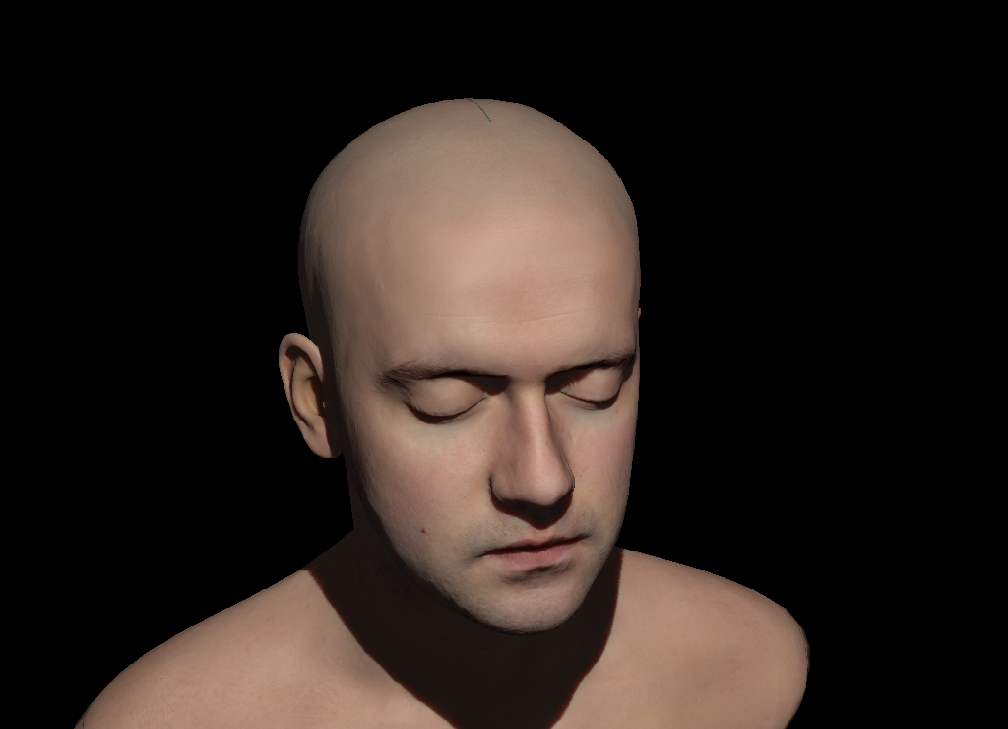
Evaluation
The result of the implementation can be seen in Figure 3 and Figure 4. The first figure shows the result of rendering with frontal lighting wheres the second shows the same situation with a light behind the object. This reveals how the light shines through thin parts of the objects at the ear.
The resulting image still has the problem of a visible texture seam (see Figure 5) which originates from blurring across texture chart borders, i.e. the blur passes consider texels which are not mapped to any location on the geometry. Those pixels are black and therefore the seams appear as dark lines. This can be fixed relatively easy by ignoring such texels. This requires some way of determining which texels of the irradiance map are at the seams which could be done via the alpha channel. However, the alpha channel is already occupied with the thickness value to determine light that shines through the object. In consequence another texture, possibly the stencil buffer, could be used at the expense of another texture fetch.
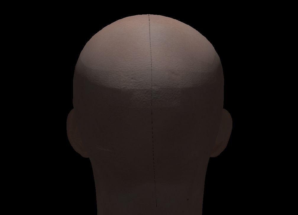
Image quality is also degraded by the lack of anti-aliasing which is very apparent at the edges of the head and the nose in Figure 3. Adding anti-aliasing is not too difficult in this case as the image is forward rendered and could therefore make use of the hardware supported MSAA in the final render pass.
The average measured frame time on a GeForce GTX 1060 is around 7.5ms which allows 60fps but would use up most of the available 16.6ms budget available for that frame rate. These timings would increase drastically, if more objects exposing subsurface scattering were rendered per frame. Other solutions like [JSG09]J. Jimenez, V. Sundstedt and D. Gutierrez. Screen-space Perceptual Rendering of Human Skin, 2009
http://giga.cps.unizar.es/~diegog/ficheros/pdf_papers/TAP_Jimenez_LR.pdf
do not suffer from this shortcoming and are therefore better suited for real time rendering. Nevertheless, the current implementation still has some room for improvement by avoiding the waste of two color channels for the shadow map for example. Reducing bit depth of render targets might be another option to increase performance. None of this had been tried as performance was acceptable for the use case already.
This project's repository is at
https://bitbucket.org/rsafarpour/texturespacediffusion