Skin Rendering with Screen Space Subsurface Scattering

Moving the subsurface scattering part into screen space means that the blur occurs relatively late in the pipeline, when all objects have been rendered into a full screen buffer. This turns subsurface scattering in a post-processing effect which significantly facilitates the whole rendering process and also simplifies integration into an existing renderer.

The first step of the algorithm is to determine irradiance at the surface. This is done using two distinct render passes: In contrast to the texture space method the first pass creates a plain shadow map, as there is no additional information needed for translucency. The following irradiance pass then calculates irradiance on the skin surface using the light source, shadow map and the surface normals. Both normals and final irradiance are determined exactly as described in the texture space method which means that irradiance is calculated via a physically based BRDF for specular reflection (here a GGX distribution with Smith shadow/masking function) and a Lambertian BRDF for diffuse reflection. This is a difference to the original description of the algorithm in [JSG09]J. Jimenez, V. Sundstedt and D. Gutierrez. Screen-space Perceptual Rendering of Human Skin, 2009
http://giga.cps.unizar.es/~diegog/ficheros/pdf_papers/TAP_Jimenez_LR.pdf
which relies on the original texture space diffusion algorithm and therefore uses the Kelemen-Szirmay-Kalos BRDF presented by [KSK01]C. Kelemen and L. Szimay-Kalos. A Microfacet Based Coupled Specular-Matte BRDF Model with Importance Sampling, 2001
http://cg.iit.bme.hu/~szirmay/scook.pdf
to calculate irradiance. This pass has two output render targets, where one receives the resulting body reflection and the other stores the resulting surface reflection. Figure 1-Figure 3 show the results of the first passes, a shadow map, a specular irradiance map and a diffuse irradiance map.

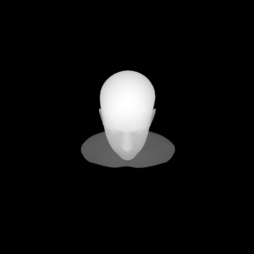
In order to perform the blur which approximates subsurface scattering, the algorithm needs a mask to identify pixels which need to be blurred. This serves two purposes: It reduces the number of pixel shader invocations, as scheduled invocations for unmasked pixels can be culled right away. The number of untouched pixels is usually quite high in typical scenarios as close ups of faces are relatively rare. This is different in the example application which focuses the camera on one face to be rendered to demonstrate the effect. The other reason for the render mask is correctness as other surfaces must not be blurred. Even if there are no other objects in the final image, as in the example, the mask is needed to prevent halos. See Figure 4 for the mask and Figure 5 for rendering without a mask.

The mask itself is generated in a dedicated pass by issuing draw calls without any bound render target and depth testing disabled. The pass only writes the configured stencil reference value into the stencil buffer and is therefore very fast. An alternative would be to generate the mask in the irradiance pass to save some more time. The final pass then draws a full screen quad while the stencil test only passes for pixels for which the stencil buffer value has been set. This is the same pass which performs the blur described next.

Jorge Jiminez et al. [JSG09]J. Jimenez, V. Sundstedt and D. Gutierrez. Screen-space Perceptual Rendering of Human Skin, 2009
http://giga.cps.unizar.es/~diegog/ficheros/pdf_papers/TAP_Jimenez_LR.pdf
describe a way of approximating the scattering described by a diffusion profile. Their idea is based on the optimisations proposed for the texture space as presented by [HBH09]J. Hable, G. Borshukow and J. Hejl. Fast Skin Shading, 2009 . They approximate the full diffusion profile blur by combining a small number of samples in texture space. Their samples locations are shown in Listing 1

The first location samples irradiance at the location of the fragment to be shaded, i.e. represents direct irradiance from the light source before any subsurface scattering occurs. The other sample positions have been derived by forming two rings around the origin and splitting each ring into 6 segments. The individual positions are random locations in one of the twelve resulting segments. These jittered samples are then weighted and summed to estimate the influence of subsurface scattering.

The individual weights are shown in Listing 2 and have been derived via the known approximation of the multipole diffusion by applying a sum of Gaussians. It is explained in [HBH09]J. Hable, G. Borshukow and J. Hejl. Fast Skin Shading, 2009 .

As mentioned before this process was developed for texture space diffusion, therefore some modification is necessary to assure that the approximation is still valid in screen space. The issue is that screen space does not take depth into account by default, i.e. that fragements which are close in screen space are not necessarily close in view space and therefore the sample distribution needs to be scaled. For example, if there is a large depth difference in x direction the x-axis distance of individual samples needs to be scaled down so that distance in view space is close to constant. This is equivalent to a configuration where the sample was placed on a plane which is oriented in the direction of the surface normal. Another effect is that for fragments with a large distance the kernel needs to shrink uniformly to guarantee constant distances in view space (because objects with a larger camera distance are scaled down by the projection). Therefore the kernel needs to be scaled inversely and uniformly with distance. With increasing rate of change of distance with respect to x- and y-direction the kernel also needs to be scaled inversely along the respective axis, i.e. if the distance increases a lot along the x axis, the kernel must be scaled down in x-direction. The rate of change is the derivative of view space depth and can be obtained by unprojecting the depth buffer before using ddx(depthVS)/ddy(depthVS). The unprojection and following determination of the derivatives is shown in Listing 3

Two additional parameters are introduced to allow tuning. The first parameter $\alpha$ which is called bias in the example application, controls view space size of the kernel and the other parameter $\beta$ scales the influence of the depth derivative (the application controls therefore refer to it as scale). The final coefficient to scale the kernel in screen space x-direction is calculated as shown in Equation $(\ref{eq:kernel_scale})$, the coefficent for screen space y-direction is almost the same but uses the other view space depth derivative.

$$s_x = \frac{\alpha}{z + \beta \cdot \left|\frac{dz}{dx}\right|}\tag{1}\label{eq:kernel_scale}$$

Translucency allows light to be transmitted through thin body parts such as ears. The algorithm presented so far does not take this effect into account. The texture space method required a special shadow map to achieve this effect and blurred the resulting thickness of material when approximating subsurface scattering. By moving to screen space there's no texture space blurring and therefore this approach is not possible any more. This means that the effect must be recreated in screen space and [JWSG10]J. Jimenez, D. Whelan, V. Sundstedt and D. Gutierrez. Real-Time Realistic Skin Translucency, 2010
http://giga.cps.unizar.es/~diegog/ficheros/pdf_papers/Jimenez_skin_IEEE.pdf
describes how to achieve that. The basic idea of the method is to estimate how much radiance arrives on the surface of the back and attenuating this by the distance the light needs to travel through material, while neglecting any diffusion. The transmitted irradiance is added to the calculated irradiance at the front so that it is blurred when performing the screen space diffusion approximation later.

Since there's no information about irradiance on the back side it is necessary to make some assumptions about its surface. Specifically surface normal direction and surface albedo are unknown and absolutely necessary to evaluate the BRDF. The missing normal is estimated to be the exact opposite of the front facing vertex normal. In most cases the difference between this estimate and the actual vertex normal on the back is negligible, so that the resulting errors remain undetected by observers. Resorting to vertex normals as an estimate neglects high frequency normals from the height map, which represent surface details. This proves to be irrelevant in practice as the diffusion is effectively a low pass filter for radiance and therefore removes the effects of those detailed normals anyway.

Albedo is approximated in a similar fashion by assuming it is mostly constant for the whole object and therefore albedo on the back is estimated to be the same as on the front. This is obviously incorrect but for human skin the albedo values are always very similar. Therefore the error is very small and will be hidden after transmission and diffusion, which is why this assumption works well in the vast majority of cases.

The estimated surface normal and albedo values are then used to calculate irradiance at the back by using Equation $(\ref{eq:translucent_irradiance})$. With $\mathbf{l}$ being the light vector pointing towards the light source and $x^+$ denoting that the result is clamped to the range [0,1]. In the implementation this value is modified by subtracting a value of 0.33 to avoid unpleaseant transitions and translucency at high curvature locations (e.g. the tip of the nose). This also attenuates translucency a little more but the resulting image looks convincing.

$$ E_{back} = (-\mathbf{n}_{front} \cdot \mathbf{l})^+\tag{2}\label{eq:translucent_irradiance}$$

Knowing irradiance at the back, distance travelled through the material still needs to be determined. This is a challenge since there's no information about the back side location during post-processing render passes. Fortunately, there are only two possible lighting states for the back: Either it is not lit and irradiance at the back is zero, i.e. transmitted radiance is also zero, or it is lit and therefore some location information of the back is guaranteed to be stored in the shadow map. The information the shadow map holds is the exact position in light space, which allows to calculate the distance between the back and the front. This is done by transforming the fragment's position into light view space, unprojecting the shadow map texel into light view space and then evaluating the distance between the two points in this common space. The code to calculate this distance is shown in Listing 4. The determined distance is exact if the geometry of the scene is convex, otherwise material thickness may be overestimated as the shadow map cannot account for cavities.

With normals, albedo and travelled distance at hand, irradiance and its diffusion can be evaluated. In order to formulate that diffusion, consider transmission behaviour of irradiance from the back to the front with subsurface scattering: The exiting radiance at one point on the front depends on incoming radiance at all points on the back and is attenuated while travelling through the material towards the exit point. The attenuation is a function of distance and frequency as described by the diffusion profile. Looking at Figure 6 one can see that the distance can be calculated by the Pythagorean theorem via the distance between front and back surface d and tangential distance r.

For points with the same tangential distance r, attenuation is identic due to the assumption of perfectly parallel surfaces. This and the fact that we consider irradiance E to be constant allows to integrate irradiance over circles around the point on the back that is exactly opposite of the point being shaded. Mathematically, this is expressed in Equation $(\ref{eq:translucent_integral})$ where E was moved out of the integral based on its constancy while 2πr remains inside to simplify later.

$$L_{trans} = E \int_0^\infty 2\pi r R(\sqrt{r^2 + d^2}) \ dr\tag{3}\label{eq:translucent_integral}$$

Remembering Equation $(\ref{eq:translucent_diffusion})$ from the previous post the integral can be transformed into Equation $(\ref{eq:translucent_approximation})$ by plugging Equation $(\ref {eq:translucent_diffusion})$ in Equation $( \ref{eq:translucent_integral})$.

$$R(\sqrt{r^2 + d^2}) = \sum_{i=0}^k w_i e^{-d^2/v_i} G(v_i, r)\tag{4}\label{eq:translucent_diffusion}$$

$$L_{trans} = E \int_0^\infty 2\pi r \sum_{i=0}^k w_i e^{-d^2/v_i} G(V_i, r) \ dr \tag{5}\label{eq:translucent_approximation}$$

At this point the integral and sum can be switched and the whole expression can be reformulated as shown in $(\ref{eq:trans_approx_simplification2})$ where only the normalised Gaussian is left as an integrand which is defined to integrate to 1. Therefore the result is unaffected by the integral and it can simply be omitted. These simplifications eventually result in Equation $(\ref{eq:trans_approx_simplification3})$. The resulting radiance is then added to the reflected radiance at the front before blurring.

$$\begin{align}
L_{trans} &= E \int_0^\infty 2\pi r \sum_{i=0}^k w_i e^{-d^2/v_i} G(V_i, r) \ dr\tag{6}\label{eq:trans_approx_simplification1}\\
&= E \sum_{i=0}^k w_i e^{-d^2/v_i} \int_0^\infty 2 \pi rG(V_i, r) \ dr \tag{7}\label{eq:trans_approx_simplification2} \\
&= E \sum_{i=0}^k w_i e^{-d^2/v_i} \tag{8}\label{eq:trans_approx_simplification3}
\end{align}
$$

Since the presented implementation is based on the texture space diffusion implementation, it suffers from the same deficits (cf. conclusion section of that post). Those issues are no specular aliasing resolution, an overly simplistic shadow mapping algorithm, a missing bloom effect, missing ambient occlusion and no tone mapping. As for the texture space diffusion these problems are not too relevant for this demo and therefore haven't been resolved.

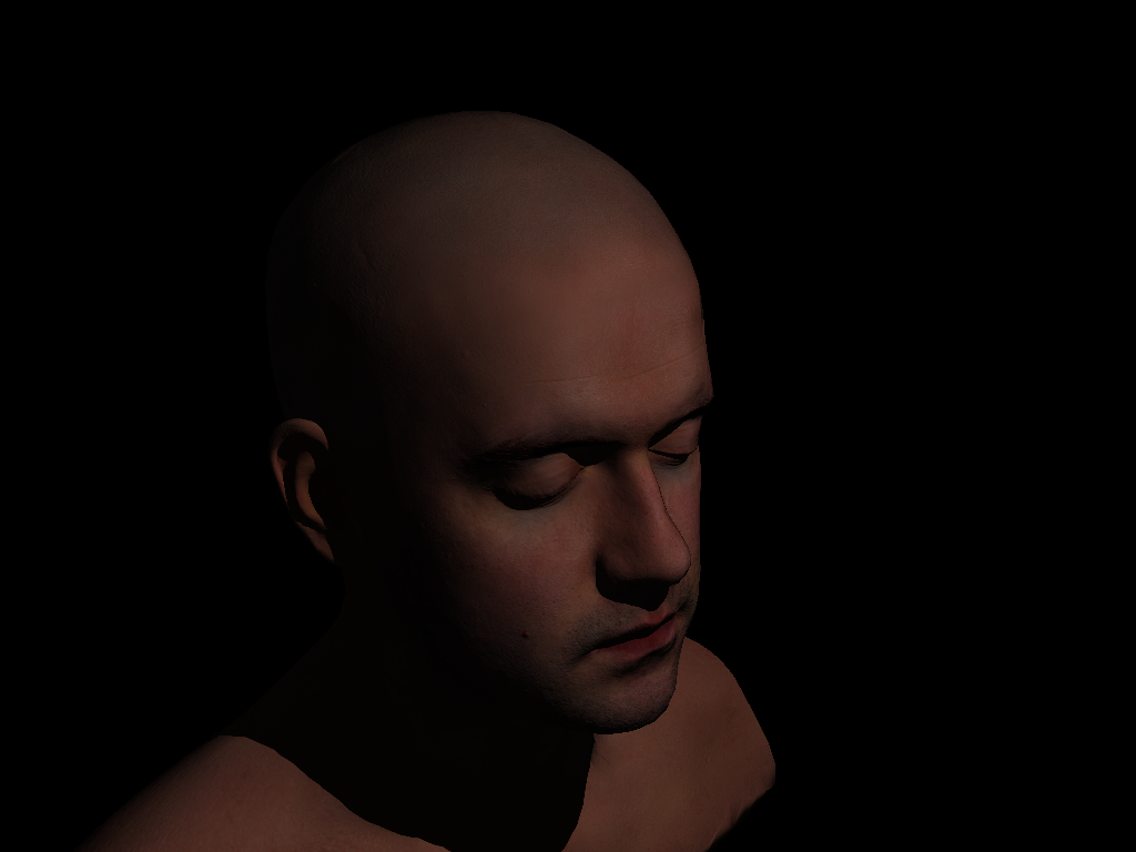
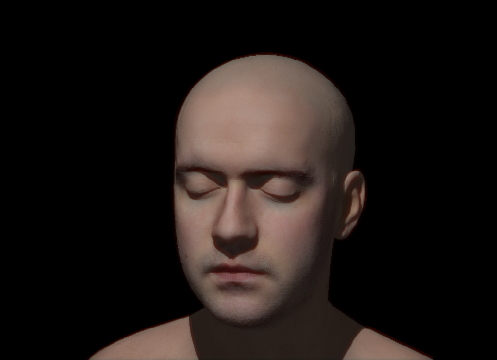
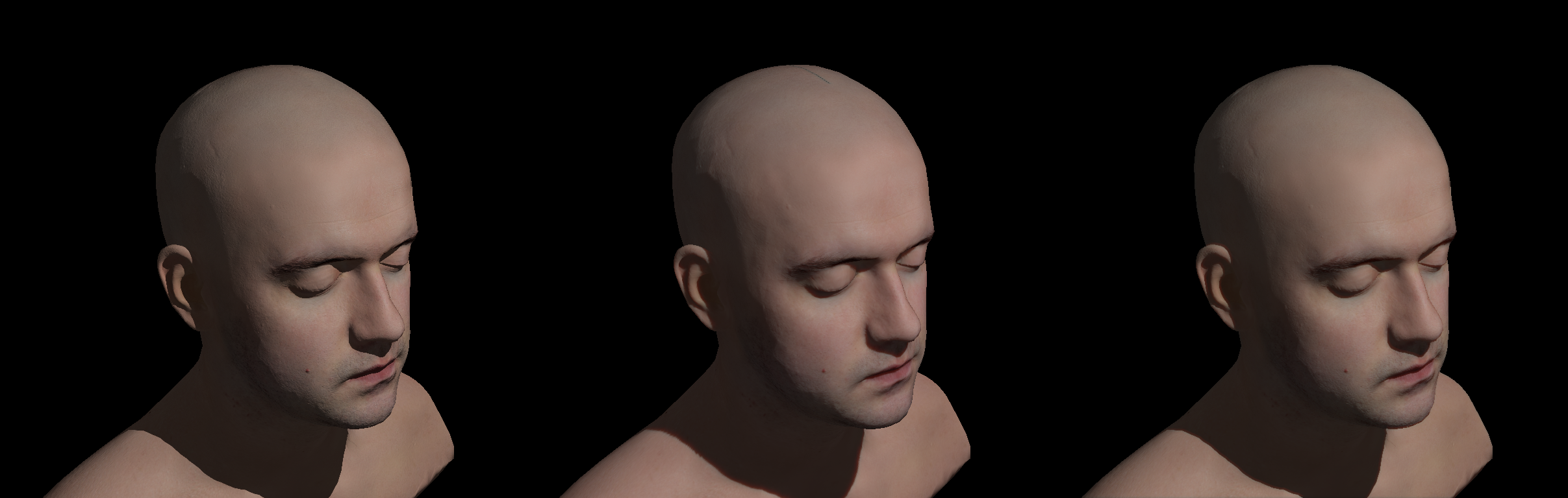
The final rendering is shown in Figure 7, while Figure 8 compares the results of screen space subsurface scattering and texture space diffusion to no subsurface scattering. It is apparent that a similar effect at a slightly lower quality can be achieved using the screen space method while it provides significant performance advantages. While texture space diffusion takes approximately 7.5ms per frame on a GeForce GTX 1060 the screen space approximation runs at slightly below 1.5ms per frame. This is a fifth of time the former method needs even though the scene puts the screen space method at a disadvantage. The head model covers a large part of the screen while ususal scenes would have much less screen coverage for objects exposing the effect. This means that for most scenes less pixel shaders are invoked to produce the effect which would reduce frame time even further. For the texture space method, performance does not scale with screen coverage so that the performance gap would only grow in most realistic scenes.

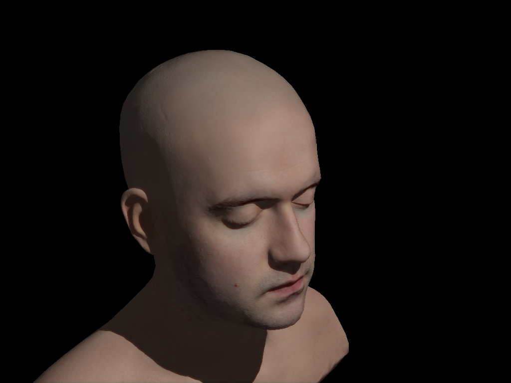
In Figure 9 the effect of skin translucency is shown. The presented translucency algorithm does provide a convincing effect which is less correct than the one created via texture space but the error is difficult to detect.

Unfortunately the seam problem at the back is still present but this time it is not a inherent issue of the skin rendering method but most likely caused by the normal extraction algorithm. This algorithm takes the neighboring texels to generate a normal from a heightmap using central differences which fails at heightmap boundaries.

Two different skin rendering algorithms were presented here, which does not cover all possible approaches. Beyond texture space and screen space approximations it is possible to add the effect of subsurface scattering by using pre-integration. This technique is explained extensively by Matt Pettineo in this post.

The demo application code is here:
https://bitbucket.org/rsafarpour/texturespacediffusion